Quick Start

CuGBasis is suitable for the evaluation of the electron density and its various derivatives of interest for the quantum chemistry community. It offers an easy to use functionality, being highly applicable to larger systems, and can read various popular wave-function formats. This example will illustrate various different post-processing tools that cuGBasis can be used for.

Installation cuGBasis on Colab

The user can skip this step if they aren’t using Google Colab.

Installation of cuGBasis is rather simple, given that the user has CMake, and CUDA installed.

Enable GPU

On Google Colab, the GPU needs to be enabled. The user should do the following:

Click on Runtime -> Change runtime type -> T4 GPU

#@title **Installing Horton, ChemTools and cuGBasis
#@markdown It may take a few minutes! Make sure to enable GPU
!pip install -q condacolab
import condacolab
condacolab.install()
!pip install numpy scipy pybind11 qc-iodata
!pip install git+https://github.com/theochem/grid.git
!mamba install -c theochem horton
!pip install git+https://github.com/theochem/chemtools.git
!git clone https://www.github.com/theochem/cuGBasis
%cd cuGBasis
!git submodule update --init --recursive
!ls
!pip install -v .
%cd examples/

Constructing Molecule Object

The first-step is to read the wave-function file and constructing the Molecule class.

%cd ./cuGBasis/examples/
from cugbasis import Molecule

file_path = r"./ALA_ALA_peptide_uwb97xd_def2svpd.fchk"
mol = Molecule(file_path)

[Errno 2] No such file or directory: './cuGBasis/examples/'
/home/ali-tehrani/SoftwareProjects/cugbasis/examples

Electron Density

The molecule class can efficiently calculate the electron density. These examples will use Grid package to construct various grids for evaluation.

Molecular Integration and Dipole Moment

The integration of the electron density

\[\int \rho(\mathbf{r}) d\mathbf{r} = N\]

should provide the total number of electrons. This example will construct a Becke-Lebedev grid using MolGrid object from grid package using Hirshfeld atom-in molecules weights. Additionally, it will calculate the dipole moment of this peptide.

import numpy as np
from grid.molgrid import MolGrid
from grid.hirshfeld import HirshfeldWeights
from grid.utils import dipole_moment_of_molecule

# Construct Molecular Grid
atom_numbers = mol.atnums     # Atomic numbers
atom_coords = mol.atcoords    # Atomic coordinates
molgrid = MolGrid.from_preset(atom_numbers, atom_coords, preset="fine", aim_weights=HirshfeldWeights())

# Calculate density over grid
density = mol.compute_density(molgrid.points)

print(f"Total number of electrons:       {np.sum(atom_numbers)}")
print(f"Integration of electron density: {molgrid.integrate(density)}")

# Calculate Dipole Moment
dipole = dipole_moment_of_molecule(molgrid, density, atom_coords, atom_numbers)

print(f"Dipole Moment: {dipole}")

/home/ali-tehrani/miniconda2/envs/py37/lib/python3.7/site-packages/grid/atomgrid.py:896: UserWarning: Lebedev weights are negative which can introduce round-off errors.
  sphere_grid = AngularGrid(degree=deg_i, method=method)

Total number of electrons:       108
Integration of electron density: 107.99956413601713
Dipole Moment: [-1.19887145  1.57689994 -1.90832791]

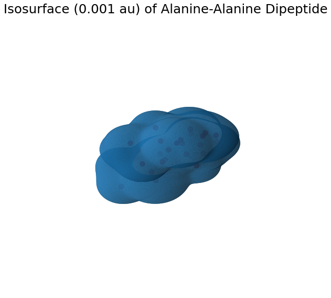
Isosurface and Cube Files

This example will calculate the isosurface of the electron density. Grid package is used to construct an uniform grid around the molecule from which an isosurface is obtained from skimage marching cubes implementation.

from grid.cubic import UniformGrid

grid = UniformGrid.from_molecule(atom_numbers, atom_coords, spacing=0.1, extension=8.0)
print(f"Cubic Grid Shape: {grid.shape}")
print(f"Number of Points: {len(grid.points)}")

dens = mol.compute_density(grid.points)

# Optional: Save the cube file
#grid.generate_cube("./density_ALA_ALA.cube", dens, mol.coordinates, mol.numbers)

Cubic Grid Shape: [322 279 218]
Number of Points: 19584684

import numpy as np
from skimage.measure import marching_cubes

# Reshape density to have the cubic shape (N_x, N_y, N_z) for marching cubes
dens_shaped = dens.reshape(grid.shape)

# Run marching cubes algorithm
kverts, kfaces, _, _ = marching_cubes(dens_shaped, 0.1, allow_degenerate=False)
kverts = kverts.dot(grid.axes) + grid.origin
print(f"Number of vertices: {len(kverts)}")

# Compute the density again on the isosurface to validate it
dens_iso = mol.compute_density(kverts)
print(f"Mean Density on isosurface: {np.mean(dens_iso)}")
print(f"STD  Density on isosurface: {np.std(dens_iso)}")

Number of vertices: 59974
Mean Density on isosurface: 0.09988541206828618
STD  Density on isosurface: 0.00016651218345750148

%matplotlib qt
import matplotlib.pyplot as plt
import matplotlib
matplotlib.use("qt5agg")
fig = plt.figure(figsize=(10, 10))
ax = fig.add_subplot(projection="3d")
ax.plot_trisurf(kverts[:, 0], kverts[:, 1], kverts[:, 2], triangles=kfaces)
ax.scatter(atom_coords[:, 0], atom_coords[:, 1], atom_coords[:, 2], color="r", s=100)
plt.axis("off")
plt.title("Isosurface (0.001 au) of Alanine-Alanine Dipeptide", fontsize=25)
plt.show()

elec = mol.compute_electrostatic_potential(kverts[np.random.choice(np.arange(len(kverts)), 5000)])

print(np.max(elec))
print(np.mean(elec))

2.5024174500632683
0.8277023718436348

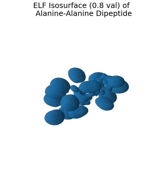
Electron Localization Function (ELF)

from chemtools.toolbox.interactions import ELF
from skimage.measure import marching_cubes

grid = UniformGrid.from_molecule(atom_numbers, atom_coords, spacing=0.25, extension=8.0)
print(f"Cubic Grid Shape: {grid.shape}")
print(f"Number of Points: {len(grid.points)}")

dens = mol.compute_density(grid.points)

# Evaluate quantities for Electron Localization Function
grad = mol.compute_gradient(grid.points)
ked = mol.compute_positive_definite_kinetic_energy_density(grid.points)

elf = ELF(dens, grad, ked, grid=grid, trans="rational", trans_k=2, trans_a=1, denscut=0.0005)

# Optional: create cube files
#grid.generate_cube("elf_ALA_ALA.cube", elf.value, mol.coordinates, mol.numbers)

# Optional: create vmd file for visualization
#elf.generate_scripts("elf_ALA_ALA.vmd", isosurf=0.8)

# Run marching cubes algorithm for generating isosurface
elf_vals = elf.value.reshape(grid.shape)
kverts, kfaces, _, _ = marching_cubes(elf_vals, 0.8, allow_degenerate=False)
kverts = kverts.dot(grid.axes) + grid.origin
print(f"Number of vertices: {len(kverts)}")

Cubic Grid Shape: [129 112  87]
Number of Points: 1256976
Number of vertices: 17591

%matplotlib inline
import matplotlib.pyplot as plt

fig = plt.figure(figsize=(10, 10))
ax = fig.add_subplot(projection="3d")
ax.plot_trisurf(kverts[:, 0], kverts[:, 1], kverts[:, 2], triangles=kfaces)
ax.scatter(atom_coords[:, 0], atom_coords[:, 1], atom_coords[:, 2], color="r", s=100)
plt.axis("off")
plt.title("ELF Isosurface (0.8 val) of \n Alanine-Alanine Dipeptide", fontsize=25)
plt.show()

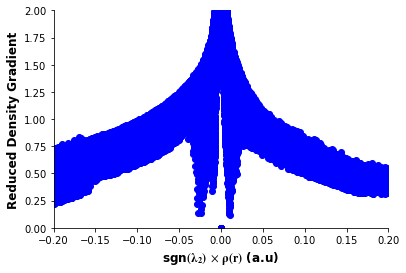
Non-Covalent Interactions (NCI)

%matplotlib inline
from chemtools.toolbox.interactions import NCI

# Evaluate quantities for Electron Localization Function
density = mol.compute_density(grid.points)
rdg = mol.compute_reduced_density_gradient(grid.points)
hessian = mol.compute_hessian(grid.points)

nci = NCI(density, rdg, grid=grid, hessian=hessian)

# Optional: create vmd file for visualization
#nci.generate_scripts("nci_ALA_ALA.vmd", isosurf=0.5, denscut=0.05)

# Create plot
nci.generate_plot("nci_ALA_ALA.png")

findfont: Font family ['serif'] not found. Falling back to DejaVu Sans.
findfont: Font family ['serif'] not found. Falling back to DejaVu Sans.